Atomic force microscopy has the capacity to identify a range of nanoscale properties alongside topography in any environment; this is central to the power and extensive applicability of this method.
While accessing properties in the realms of electrical, chemical, thermal, and electrochemical measurements is common, the atomic force microscope (AFM) is particularly known for its distinct ability to measure mechanical properties. This is thanks to the diverse range of options when it comes to the interaction between the AFM probe and sample set-up and measurement approaches.
This article offers an summary of nanomechanical characterization using an AFM, with a focus on measurements of the most relevant and wide-ranging mechanical properties found on the nanoscale, including viscoelastic properties, elastic modulus, adhesion and friction.
Nanomechanical Modes of Operation
Developed over 30 years ago, AFM quickly gained recognition for a mechanical contrast technique called phase imaging. This measurement, inherent to the tapping mode, produces contrast drawn from a range of mixed mechanical properties.
However, the measurements detailed in this article go beyond general mechanical contrast, offering both semi-quantitative and quantitative information about individual mechanical properties.
The multitude of three- or four-letter acronyms referring to mechanical modes in scanning probes and atomic force microscopy can be challenging to navigate. One effective way to categorize the various modes is by considering the type of AFM tip-sample interaction.
Using this approach, the various modes can be categorized into three main types:
- Resonance: The tip is oscillating at its cantilever’s resonance frequency.
- Off-Resonance: The tip is oscillating at a frequency that is not its cantilever’s resonance frequency.
- Contact: The tip/cantilever does not oscillate, but, when the tip comes into contact with the sample, a non-periodic deflection is observed.
Based on this categorization, a non-exhaustive list of the various modes is organized in Table 1, illustrating which modes can measure individual properties.
Table 1. Overview of nanomechanical AFM modes and the mechanical properties they can measure. *Phase contrast provides a single signal that is a convolution of elastic modulus, viscoelastic modulus, and adhesion. Source: Bruker Nano Surfaces and Metrology
| Resonance Category |
Description |
Elastic Modulus, Stiffness, Deformation |
Viscoelastic Loss Modulus, Tan Delta |
Adhesion |
Friction |
Plastic Deformation and Creep |
Reference |
| Contact |
Lateral force microscopy (LFM) |
|
|
|
 |
|
|
| Resonance |
TappingMode with phase contrast (Phase imaging) |
* |
|
|
|
| Torsional resonance mode (TR-Mode) |
|
|
|
|
|
|
| Contact resonance |
|
|
|
|
|
B. Pittenger and D. Yablon. (2017). Bruker Application Note 148 |
| Off-resonance |
Force spectroscopy (Force-distance) |
|
|
|
|
|
|
| Force volume |
|
|
|
|
|
|
| PeakForce quantitative nanomechanics (PeakForce QNM) |
|
|
|
|
|
B. Pittenger, S. Osechinskiy, and D. Yablon. (2019). Bruker Application Note 149 |
| Ringing mode |
|
|
|
|
|
M.E. Dokukin and I. Sokolov. (2017). Scientific Reports 7(1):11828. DOI: 10.1038/s41598-017-12032-z |
| AFM-based nanoscale dynamic mechanical analysis (AFM-nDMA) |
|
|
|
|
|
B. Pittenger and D. Yablon. (2017). Bruker Application Note 154 |
Elastic Modulus
The most sought-after mechanical measurement on the nanoscale is stiffness, typically expressed as an elastic modulus (also known as Young’s modulus). The elastic modulus quantifies elastic deformation within a regime where the material is still stretching, and the motion remains reversible, occurring before any irreversible deformation or deterioration sets in.
In bulk materials, the elastic modulus is measured experimentally by fitting the initial linear region of a stress vs. strain plot.
On the microscale, aside from an instrumented nanoindenter, the AFM is the only instrument capable of measuring elastic modulus.
It is the only instrument capable of performing these measurements on truly small length scales (tens of nm laterally, a few nm in depth) and on very soft materials with moduli as low as kPa.
As shown in Table 1, many AFM modes have been developed to measure elastic modulus, including force volume, force-distance curves, PeakForce QNM®, AFM-nDMA, Ringing Mode, and contact resonance.
Figure 1 illustrates PeakForce QNM measurements of the moduli for a blend of rubber, polypropylene (PP), polyethylene (PE), and nanoparticles.
In PeakForce QNM, the tip moves in and out of the surface, with the force continuously measured throughout both the approach and retract cycles.
Unlike force volume and force-distance curves that operate on a linear ramp, PeakForce QNM uses a sinusoidal ramp to move the tip in and out of the surface, allowing for faster and more controlled measurements.
Mechanical properties are extracted from the force vs. tip-sample separation measurement plots using different models that account for various forms of adhesion, such as the Johnson-Kendall-Roberts (JKR) and Derjaguin-Muller-Toporov (DMT) models.
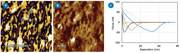
Figure 1. PeakForce QNM image (15 μm scan size) of a heterogeneous polymer blend, showing (a) LogDMTModulus, (b) height, and (c) individual force vs tip-sample distance curves. The four materials are easily differentiated by contrast in (a) and (c): nanoparticles (dark blue) rubber (light blue), polyethylene (gray), and polypropylene (orange). Dotted lines indicate approach and solid lines indicate retract. Image Credit: Bruker Nano Surfaces and Metrology
PeakForce QNM can easily distinguish between the four different components, with the topography illustrated in the middle and the LogDMTModulus channel displayed on the left. DMT relates to the DMT model applied to ‘fit’ the data; the moduli are then shown on a log plot for easier visualization.
Individual PeakForce QNM curves from the various components are displayed on the right, with the dark blue cross showing a nanoparticle measurement. The orange cross relates to a PP domain, while the gray and light blue show a PE domain and a rubber domain, respectively. The slopes of each individual curve, from which the elastic modulus is measured, are easily distinguished in the plots.
Viscoelastic Moduli
Viscoelastic materials refers to materials whose modulus is contingent on the frequency at which it is being measured. Silly Putty is a well-known example of such a material, where stiffness is determined by how fast (the frequency) at which it is stretched. However, there are many more sophisticated examples, particularly among polymers and biological materials.
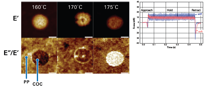
Figure 2. AFM-nDMA scans (left, 2 μm scans each) showing storage modulus (E', top row) and loss tangent (E''/E', bottom row) of a blend of polypropylene (PP) and cyclic olefin copolymer (COC) as a function of temperature. A pair of AFM-nDMA ramps (right) collected on a stiff (blue) and a soft (pink) material, showing the small amplitude oscillation during the hold segment. Image Credit: Bruker Nano Surfaces and Metrology
There are three major viscoelastic moduli, each of which is a function of frequency and temperature:
- Loss modulus E” (dissipated energy)
- Loss tangent tan δ (also called tan delta, ratio of loss modulus/storage modulus)
- The storage modulus E’ (elastically stored energy)
Viscoelastic moduli are crucial for predicting and understanding a material’s performance. For example, the loss tangent is used as a performance metric for tires, and loss tangent vs. temperature plots are used to measure glass transition temperatures.
There are two primary methods used for measuring viscoelastic moduli with AFM: contact resonance and AFM-nDMA.
With contact resonance, the measurement frequency is contingent on the resonant frequency of the cantilever in contact with the sample, usually hundreds of kilohertz to megahertz. Comparatively, when using AFM-nDMA, the resonance is not applied, so maps or point spectra can be collated.
Each measurement involves a hold period with modulation at a fixed amplitude and a user-defined frequency or range of frequencies, which can vary from 0.1 Hz to 20,000 Hz. During the modulation segment, amplitude and phase data are analyzed to calculate the three viscoelastic properties: E', E'', and loss tangent.
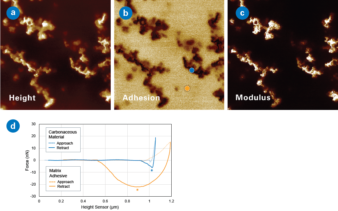
Figure 3. Force volume scans (2 μm) showing (a) height, (b) adhesion, and (c) modulus. Individual force curves at locations indicated in (b) are plotted in (d), showing the carbonaceous material (blue) having low adhesion and the matrix adhesive material (orange) having high adhesion. An asterisk marks the adhesion dip for each material. As seen in the force curves, bright areas in the adhesion map (b) correspond to about 20-30 nN of adhesion, while dark areas have adhesion of <10 nN. Image Credit: Bruker Nano Surfaces and Metrology
AFM-nDMA has the capacity to measure these properties as a function of frequency or temperature, as displayed in Figure 2 of the mixture comprised of polypropylene (PP) in the matrix and cyclic olefin copolymer (COC) in an island in the middle.
The mixture is then measured as a function of temperature at room temperature, where the storage modulus E’ of the two materials remains fairly constant until reaching a temperature of around 175°C.
As displayed in these 2x2 µm2 images, the polypropylene matrix then softens faster than the COC, as seen in the E’ map on top, while the loss tangent contrast inverts as the temperature nears the glass transition of the COC.
Adhesion
As the tip comes into mechanical contact with the surface, it frequently adheres to the sample due to local attractive forces. As the tip retracts, the adhesion force can be measured using different methods, as displayed in Table 1.
A popular method to measure adhesion is through force spectroscopy, which includes individual force-distance curves or a map of such curves that, when collected together, form a force volume data cube. An individual force curve can be analyzed for various properties, including adhesion and modulus, the latter of which is modeled using different contact mechanics models. Force volume provides mapping capability, allowing the distribution of properties to be easily visualized.
A force volume map of a carbon sticky stub commonly used to secure samples is shown in Figure 3, with height (left), adhesion (middle), and modulus (right) maps, all extracted from fitting individual force curve data.
The AFM images reveal two distinct areas: the matrix, which dominates the sample and has high adhesion but is soft (this is the “glue” in the sticky stub), and patches of non-sticky, hard material (the carbonaceous material).
Individual force curves are shown at the bottom. The force curves from the carbon material (blue dot) correspond to the dotted blue/solid blue approach/retract force curves, showing a minimal adhesion dip (marked by an *) as the tip retracts from the surface.
In contrast, a force curve from the matrix (orange dot on the adhesion map) corresponds to the dotted orange/solid orange approach/retract force curves, showing a very large adhesive dip as the tip retracts from the surface.
Friction
As measured by AFM, friction refers to the force that resists the relative motion of the tip and substrate as the tip moves parallel to the surface. Friction force can be calculated via lateral force mode when there is contact between the tip and the sample, which is then scanned in a direction perpendicular to its cantilever axis.
Consequently, the normal force (i.e., the force exerted by the cantilever) is known, and the friction force can be determined by observing the twisting motion of the cantilever as it scans across a surface.
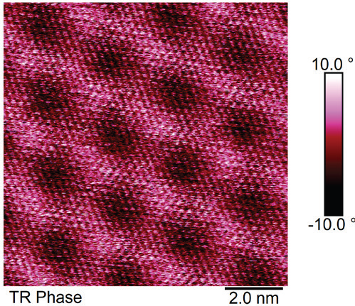
Figure 4. Torsional resonance force microscopy phase channel image of a moiré superlattice formed between monolayer graphene and hBN with a period measuring 2.6 nm. Adapted from M. Pendharkar, S.J. Tran, G. Zaborski, et al. (2024). DOI: 10.1073/pnas.2314083121, licensed under CC BY.
Torsional force dynamic friction microscopy (TR-DFM) is an alternative technique that is sensitive to a relative force termed dynamic friction.
During the application of this mode, the cantilever is positioned so that it is in direct contact with the surface and then oscillates side-to-side at its torsional contact resonance frequency. This is in contrast to the aforementioned “traditional” cantilever resonance modes, where the cantilever is oscillated perpendicular to the surface.
The phase of this torsional resonance can then be measured and exhibits sensitivity to the mechanical dynamic friction of the surface. An image of the torsional phase of a monolayer of graphene on hexagonal boron nitride (hBN) is displayed in Figure 4.
The atomic lattice of hBN is easily observed, with the finer features likely corresponding to the underlying graphene lattice. A moiré period of 2.6 nm is measured, indicating a relative twist of 5.4° between the monolayer graphene and hBN.
Experimental Considerations
While making qualitative comparisons of mechanical properties across a sample can be relatively simple, quantitative nanomechanical measurements with AFM do necessitate careful probe selection alongside a meticulous calibration of both the cantilever spring constant and tip radius.
The cantilever is usually selected on the basis of its spring constant or stiffness. The cantilever stiffness must be a general match to that of the sample in order to possess the appropriate level of sensitivity to probe the sample.
The tip radius must be determined, as this is a key parameter that feeds into the different contact mechanics models. While calibration of these parameters can be conducted by the user, commercial probes now come fitted with pre-calibrated spring constants and tips with a spherical geometry whose radii are already known.
Conclusion
Atomic force microscopy facilitates crucial nanomechanical characterization capabilities that surpass simple material contrasts. AFM has an extensive range of modes available to probe a number of different mechanical properties, such as elastic modulus, viscoelastic moduli, friction, and adhesion.
All these properties are simultaneously measured on the nanoscale, with topography reaching lateral scales down to a few nm and vertical length scales of less than a nanometer.
AFM remains a powerful, versatile tool that can measure these properties in environments ranging from ultrahigh vacuums to liquids; in the arsenal of nanomechanical methods, AFM is the only one that can readily access each of these properties on the single nanometer length scale.

This information has been sourced, reviewed and adapted from materials provided by Bruker Nano Surfaces and Metrology.
For more information on this source, please visit Bruker Nano Surfaces and Metrology.